The Voynich manuscript – methodological harness
The first post in this series introduced the Voynich manuscript as an object. The second followed the attempts to read it, and ended with a map of nine concepts of what the text might be, from a cipher or a language in an unfamiliar script to a shorthand, a notation or writing with no message at all. The third followed fifty years of measuring it, and closed with what is beyond doubt and what is still open.
This post turns those measurements into a test. Every concept on the map is a claim about how the text came to be, and every such claim can be checked against a fixed list of measurable properties. That list, together with the rules for measuring, is what this post calls the harness: a fixed rig into which any candidate explanation can be plugged and run. Everything in it comes from published work, or is computed from published numbers and code, as marked; the software that runs it, and this blog’s own measurements of the text, come in later posts.
The post is long, because the list is long. It is built to be read in two passes:
- The short pass. Why a harness, the rules, the list at a glance, the scorecard and which metric bears on which concept. These give the whole argument.
- The long pass. The metrics one by one: for each of the 24 metrics, what it measures in plain words, the manuscript’s value, what it tells apart, and what to be careful about. It is reference material to dip into: every M-number in the tables links to its section. Then whether there is one number for all metrics, a map of the models, the open targets, what the harness cannot do and what comes next.
Why a harness
A decipherment says: apply this procedure to the text, and you get a message. A theory of meaningless text says: apply this procedure to nothing, and you get the text. A theory of a cipher says: apply this procedure to a message, and you get the text. A theory that the text is a natural language says: texts in a language of this kind, measured the same way, look like this. All four can be put to the measurements. A process can be run and its output measured; a language hypothesis is tested by measuring real texts of the proposed kind.
This figure is drawn in the browser and needs JavaScript.
Ctrl/⌘ + scroll to zoom · drag to pan · double-click to reset
Two lessons from the history of the field shaped it.
The first, from a century of failed readings, is that a claim has to be tested by a procedure, not by how plausible its output sounds. Every claimed decipherment so far has produced text that its author found convincing, and none has survived a test its author did not design.
The second, from fifty years of statistics, is that single measures settle nothing. In 2022 Daniel Gaskell and Claire Bowern asked people to write pages of meaningless text by hand, and compared them with the manuscript. By their test of similarity, at least 5% of one group’s values falling within the central 90% of the other’s, the manuscript was plausibly like the gibberish on 41 of their 42 measures and like meaningful text on 38; by the same test, the gibberish was like meaningful text on all 42. Their gibberish samples were only one to three pages long.1 Each measure taken alone can be met by very different processes. Only many measures taken together narrow the field, and only if each is measured the same way for every text.
Gaskell and Bowern already judged each measure by an explicit threshold. In 2026 three papers turned this into joint tests: lists with target values that a model has to meet together, so that a claim can actually pass or fail:
- Christophe Parisel set out four signatures of how Voynich words begin and end, “against which any future generative or cryptanalytic model of the VMS can be evaluated”, and showed that two kinds of generator could not meet them together.2
- Yang Ou proposed a “statistical Turing test”: eight measures applied at once to 18 models from nine families, run 30 times each. None passed all eight.3
- Liudmila Rozanova and Alexander Temerev built a joint profile of the text against eight prose texts and a catalogue (Linnaeus’s list of plant species), ran the two best published imitations through it, and named the properties those imitations still miss.4
Each of the three has its own strengths and blind spots, and the list below borrows from all of them because none covers everything. A table at the end of the scorecard sets their strengths and limits side by side.
Earlier frameworks came from both sides of the argument. In 2013 Diego Amancio and colleagues proposed “a framework for determining whether a text … is compatible with a natural language”, compared the manuscript with the New Testament in 15 languages on word statistics and on networks of words, and found it “mostly compatible with natural languages and incompatible with random texts”, with two exceptions: more repeated word pairs than chance, and topic words that cluster more than in their languages.5 In 2016 Gordon Rugg and Gavin Taylor worked the other way round: they took a list of the manuscript’s statistical features, among them Zipf’s law, the symmetric word lengths and the change of vocabulary through the book, and set out to reproduce them with a table of word parts and a grille, a card with holes slid over the table.6
The rules of measurement
A metric is only as good as the way it is taken. These are the rules this post draws from the recent literature, with what each one guards against. Few studies follow all of them, and almost none gives the manuscript’s own values an interval (rule 6).
| # | Rule | What goes wrong without it |
|---|---|---|
| 1 | Say what was measured: transcription, glyph inventory, space policy, which parts of the page | Numbers that cannot be compared or reproduced |
| 2 | One recipe for every text | A comparison that measures the recipes, not the texts |
| 3 | Compare with controls, not with randomness | “Not random” proved, which no one disputes |
| 4 | Test everything at once | A model tuned to each metric in turn |
| 5 | Rebuild the competition | Comparison with numbers taken under another recipe |
| 6 | Fix the tolerance in advance | Moving the goalposts after the result |
| 7 | Hold data back, and spend it once | A model that reproduces what it was fitted to |
| 8 | Take the book apart along its seams | An average over two systems that describes neither |
| 9 | Report what failed | A literature of successes only |
1. Say what was measured. The manuscript has been transcribed into Latin
letters several times, by different people, and every number about it depends
on choices made before the counting starts: which transcription, and which
version of it; whether ch is one glyph or two, and iin one or three (in
EVA, the usual way of writing the glyphs in Latin letters, ch is a single
glyph written with two letters); whether a space the transcribers marked as
uncertain counts as a space; whether labels and the writing in rings are
counted with the paragraph text. These choices move the numbers more than most
effects the field argues about: counting ch as one glyph or as two changes
how predictable the next glyph looks. A preregistered audit by Veronika Lux
this year re-measured five published claims on three transcriptions and found
exactly that.7 So every number comes with its recipe, and so does every
gap.
2. One recipe for every text. If the manuscript’s ch is counted as one
glyph, the control text is treated in the matching way, for example by counting
its common two-letter combinations as one sign as well.
3. Compare with controls, not with randomness. Showing that the text is not random proves nothing: no serious explanation says it is. The comparison that means something is with matched controls: real texts in several languages, ciphers, gibberish and the published generators, at the same length as the manuscript sample. Rozanova and Temerev went further and poured each prose control into the manuscript’s own sequence of line lengths, because several of the metrics below are properties of the line.
4. Test everything at once. A model passes only if it passes every metric together, as in Parisel’s and Ou’s tests. It is easy to build a model for any one metric; the difficulty, and the information, is in meeting all of them.
5. Rebuild the competition. A model is tested against its rivals run or rebuilt under the same recipe, not against their published numbers, as Rozanova and Temerev did with both leading generators.
6. Fix the tolerance in advance. Each value for the manuscript comes with an interval from resampling: how much the value moves when whole quires (the gatherings of folded sheets the book is bound from) or bifolia (single folded sheets) are left out at random. Leaving out single words instead would understate it, because neighbouring words are not independent. Each model is run several times with different random seeds, and what counts as a match is decided before the run.
7. Hold data back, and spend it once. A model fitted to part of the text is tested on text it has not seen: leaving whole quires out and refitting (Rozanova and Temerev), or the weaker split of fitting on the front of each leaf (folio) and testing on the back (Rod Kinnison).8 Where possible the analysis is registered before the confirmatory run, as Lux’s audit was; she is open that her tolerances were set after a pilot on the same files. A property a model was tuned to reproduce is an input of that model, not a result.
8. Take the book apart along its seams. The text is not one homogeneous stream. Prescott Currier showed in 1976 that it falls into two varieties, which he called languages A and B, differing in which glyphs and words are common. Results are reported for A and B separately, as Parisel does, and checked across sections, scribal hands (as Lisa Fagin Davis distinguishes them, an attribution Torsten Timm disputes9), and labels against paragraph text. The two languages can differ by more than half the pooled value: the coupling at word edges (M14) is 0.137 bits in language A and 0.248 in B, around a pooled 0.197, in Rozanova and Temerev’s measurement; another measure puts A above B (M14). Any measure that runs from one leaf to the next also assumes the present order of the leaves. Many bifolia are widely agreed to have been rebound out of order; how they were first arranged is disputed.10
9. Report what failed. A metric that a model misses, or a published value that cannot be reproduced, is reported as prominently as a success.
A tenth rule is this series’ own position rather than a published result: a language model’s judgement that a reading makes sense is not evidence. Producing plausible text from weak constraints is what such models are built to do.
The list at a glance
These are the metrics a modern study of the Voynich text is expected to report, and any explanation of the text has to reproduce. They run from the smallest scale to the largest: letters, words, the joins between words, and lines, pages and the book.
Values are for the manuscript, and the prose column gives the published
natural-language controls for comparison. “R&T” is Rozanova and Temerev. Their
profile is measured on the Zandbergen–Landini transcription, paragraph lines
only; words are the 32,747 forms between the transcribed spaces, certain and
uncertain alike (closing the uncertain ones leaves 30,395). Glyph-level values
count composite glyphs such as ch, sh and iin as one, except the unit
scale (M4), which is learned on the plain EVA letters. “Ou” means Yang Ou’s
values on Takahashi’s transcription. Most of Ou’s models are trained on the
manuscript itself; among them are Markov chains, which choose each next letter
or word from the one, two or three before it, with frequencies learned from
the manuscript. The two leading generators named in the
status column are the Naibbe cipher (Michael Greshko, 2025), which turns Latin
into Voynich-like text by writing each letter as one of several glyph groups
chosen by drawing cards, and Timm and Schinner’s self-citation generator, which
writes each new word by copying a nearby one with small changes; both are
described in the third post.
The last column says where the field stands: open if no tested model and none of the published language controls reaches the value; met by models or met by languages if some do; contested if the measurement or its reading is disputed. The table states targets, not yet tolerances: few of the values have a published interval, and each verdict uses the criterion of the study that measured it. Most values are pooled over Currier’s A and B.
| # | Metric | The manuscript | Prose controls | Status |
|---|---|---|---|---|
| Letters | ||||
| M1 | How predictable each glyph is from the one before | 2.69 bits (R&T) | 3.45–3.52 bits (R&T); 311 languages ≥ 2.77 | met by models; far below European prose under any recipe, just below the most predictable languages, by a margin the recipe can close or widen |
| M2 | The same, for glyphs inside words, on unseen pages | 2.01–2.19 bits | about 3.1 bits | met by a cipher (the only generator tested) |
| M3 | What a second glyph of context adds | 0.25–0.31 bits | 0.51–0.78 bits | met by a cipher, in its author’s judgement (the only generator tested); the manuscript is below every language tested |
| M4 | The size of recurring glyph groups | 32–64 merges, 88 units | · | met by models |
| Words | ||||
| M5 | Words built from parts in fixed slots | most words fit one template | · | met by a cipher built for it |
| M6 | Word lengths | narrow, nearly binomial | · | met by models; contested |
| M7 | Size of the vocabulary | 7,022 types; top 50 cover 33.2% | 3,454–11,041 types | met by languages; tuned into one generator |
| M8 | Share of word types used only once | 69.7% | 46.8–67.7% | open for models; at the top edge of eight European prose controls, without an interval |
| M9 | Slope of Zipf’s law | −0.867 (Ou) | −0.954 (English), −1.124 (Latin) | met by four Markov chains on slope and fit; English within the slope tolerance but not the fit |
| M10 | Type–token ratio, standardised | 0.550 (Ou) | 0.407–0.475; inside the range of 101 languages on a moving-window version | met by two models and by languages |
| M11 | How predictable a word is from the one before | 4.226 bits (Ou) | 4.43 bits | met by one model; the estimate mostly reflects vocabulary size |
| M12 | How few endings the words share | 50 endings cover 80% | 109–172 endings | untested on models |
| M13 | Vocabulary that differs between parts of the book | 0.535 (Ou) | 0.423–0.464 | met by models given the sections, and by random text; not diagnostic |
| Between words | ||||
| M14 | Coupling across the space between words | 0.197 bits (R&T) | 0.018–0.120 bits | open for models; above the European prose tested; one self-published cipher claims it |
| M15 | How much one word predicts the next | 0.79% | 2.02–9.72% | met by models |
| M16 | Association of adjacent words | 0.152 (Ou) | 0.256–0.295 | met by one model |
| M17 | Neighbours that differ by one glyph | 1.12 × shuffled | 0.28–0.56 × shuffled | met by self-citation |
| M18 | Neighbouring words alike in length | positive, 0.09–0.17 | mostly negative | met by gibberish, on a whole-text measure |
| M19 | Parisel’s four boundary signatures, jointly | end-to-start 71.0% (A), 64.3% (B) | end-to-start 19.8–35.5% | open: no published generator tested meets all four; untested beyond four languages |
| M20 | Two kinds of space | AUC 0.905 | · | untested on models |
| Lines, pages and the book | ||||
| M21 | The line and the paragraph as units | strong | · | open (on a weaker version, both gibberish and meaningful text plausible) |
| M22 | Currier’s two languages, A and B | sharp switch per page | · | Parisel’s switch untested on models; Ou’s form cannot fail a text without A/B structure |
| M23 | Vocabulary that follows the subject | present | English, Latin, Chinese on one information measure | met by languages on that measure; contested reading |
| M24 | Gradual drift through the book | present | · | contested reading |
“·” means no published value for the prose controls. Prose values are from the study that measured the manuscript on that row, and two values on one row can come from different recipes: on M1, R&T’s 2.69 bits and Lindemann and Bowern’s 311 languages are not measured the same way (rule 2).
Lux’s audit re-measured five of these on three transcriptions and under several counting choices. All the effects held, but the size of three of them depends on the recipe, and the cards below say by how much (M1, M9, M21; M6 held only conditionally). Only the Currier contrast (M22) passed every combination. The values have to be quoted with their recipe; the effects themselves stand.
Some classic measurements are left out. Long-range correlation through the
text and the growth of the vocabulary with the length of a sample (Heaps’ law)
have been measured on the manuscript, but not on the published models under a
common recipe, so neither yet works as a test. Exact repetition of a word, as
in qokedy qokedy, is treated under its near relative, M17.
One published property is deliberately left out. Parisel found that inside a word the glyphs fit best read from right to left, while across words the dependence runs left to right, and none of his four comparison languages shows this. He then showed that it is a side effect of the statistics of the words themselves, of the word grammar (M5), rather than a separate property, and set it aside as a test. So does this list.
The scorecard
How natural-language controls and the published models do, as reported in print. The grid summarises; the numbers behind it follow.
How to read the grid. Each cell applies the criterion of the study that measured that pairing, not one of this post’s own (the criteria are listed under the grid):
- ✓ meets it, ✗ fails it;
- ± split or undecided: the candidate comes in several variants and they disagree, for example Markov chains of some orders meet the criterion and others do not; or the measuring study disagrees with itself; or the value sits at the edge of the controls’ range with no interval; or the property was among the candidate’s design targets;
- ⊙ built in: the candidate was tuned to this property, given it, or fitted to the whole manuscript and scored on the same text, so a match is an input, not a result (rule 7);
- · not measured, or measured without a criterion that applies.
Two limits apply to every cell. No cell rests on an interval for the manuscript’s own value, so a ✓ or ✗ within about one tolerance of the edge should be read as undecided. And Ou’s tolerances are bands around the manuscript, set for models fitted to it: a single novel or Latin text falling outside them says whether that text is the manuscript, not whether the manuscript could be a text in a language, so the prose controls are not scored on his rows.
This figure is drawn in the browser and needs JavaScript.
Ctrl/⌘ + scroll to zoom · drag to pan · double-click to reset
Read down the columns, the scorecard says three things.
No published model passes everything. The Naibbe cipher and the self-citation procedure reproduce most of the letter-level metrics, the recurring units and the weak link between adjacent words. Both fall short on the coupling at word edges (M14) and on the share of words used only once (M8), and neither has been shown to produce the line (M21). The best result in Ou’s test, seven of his eight measures as his code counts them (six under the two-sided criterion his paper states11), and one of them a Currier test no text without A/B structure can fail, came from a resampler of the manuscript’s own word pairs within each section, fitted to the whole text and scored on it. It says how much of the profile word pairs and sections carry, not how the text was made.
No tested natural language passes everything either, in the small and mostly European sets published so far. The European prose controls are far above the manuscript on letter entropy (M1–M3), well above it on the dependence between adjacent words (M15), below it on edge coupling (M14) and on near-repeats (M17), and at most two points below it on single-use words (M8), a gap no study gives an interval for. On the size of the vocabulary (M7), its variety across 101 languages (M10) and the placement of topic words (M23) the manuscript falls among languages. The record-like catalogue overshoots the manuscript on edge coupling, adjacent-word dependence and near-repeats. Languages outside Europe come closer on letter entropy: none of the 311 reaches it, by a margin small enough that the way glyphs are counted could close or widen it. Languages whose spelling changes at word boundaries, or that build words from many parts, have not been tested in print.
The generators and the languages fail in different places. The generators fail where words meet and in the open vocabulary; the languages fail at the level of letters and in the link between words. That is why the harness is a joint test: either family can be made to look good on half the list.
Two warnings about counting marks. Some rows measure one property from several sides (M1–M3 are one low entropy, M15 and M16 one weak link between words, and M7, M8, M10, M11 and M13 all depend on how rich the vocabulary is), so a candidate that fails one tends to fail the others. And a column that has been measured more often collects more marks of both kinds: the prose column is the most measured, and an untested generator shows only dots.
Ou’s released results allow one more view of his part of the grid: where each of his models, and his two language controls, falls on each of his metrics, not just whether it passes.
This figure is drawn in the browser and needs JavaScript.
Ctrl/⌘ + scroll to zoom · drag to pan · double-click to reset
The numbers behind the grid
The criteria, by source:
| Source | Metrics | A candidate meets the criterion when |
|---|---|---|
| Ou | M1, M6, M9, M10, M11, M13, M16 (for models only) | the mean of its 30 runs is inside Ou’s acceptance band (his paper says on at least 15 of 30 runs; his released code, followed here, uses the mean): Zipf slope within ±0.10 and fit within ±0.05; type–token ratio and word association within ±0.02; the pattern of differences between parts within a mean absolute deviation of 0.05; letter entropy and word entropy within ±0.10 bits; for word lengths, the mean p-value of 30 Kolmogorov–Smirnov tests, a standard test of whether two distributions differ, above 0.0512. His Currier test (accuracy within 5 points) is listed under M22 but not scored: the manuscript’s classifier is 2.7 points better than always guessing B |
| Rozanova and Temerev | M1, M4, M7, M8, M14, M15, M17 | for a generator, the authors say it reproduces the property; for prose, this post’s reading of their comparisons, since they state no pass rule: the manuscript’s value lies inside the range of their eight prose controls, ± when it is at the edge without an interval |
| Kinnison | M2, M3 | the text falls in the same region of his plot of mid-word entropy against context gain as the manuscript, judged by eye |
| Lindemann and Bowern | M1 | (prose only) the manuscript’s value lies inside the range of their 311 languages |
| Bowern and Lindemann | M10 | (prose only) the manuscript’s type–token ratio in moving windows of 2,000 words lies inside the range of their 101 languages |
| Montemurro and Zanette | M23 | (prose only) the information carried by where words are placed, and the scale at which it peaks, fall among their language texts and apart from their non-language controls |
| da Silva | M12 | (prose only) the language needs about as few endings as the manuscript to cover 80% of words; provisional, from an unchecked study |
| Greshko and Rozanova and Temerev | M1 (Naibbe) | ± rather than ✓: low glyph entropy was among the targets the cipher’s precursor was tuned against |
| Parisel | M19 | all four signatures fall inside his ranges, separately for A and B |
| Gaskell and Bowern | M1, M6, M10, M17, M18, M21 | the manuscript’s distribution and the candidate’s overlap by at least 5% (their “plausible”), on their own versions of these metrics; for prose on M21 the same test against their meaningful texts, and on M18 their own wording |
| Greshko | M21 | the cipher’s author says it produces the line structure |
The numbers, with the manuscript’s value first. “·” means not measured.
| # | Manuscript | Natural-language controls | Naibbe cipher | Self-citation | Gibberish and other models |
|---|---|---|---|---|---|
| M1 | 2.69 bits (R&T); 2.11–2.48 (L&B); 2.16 (Ou, letters and spaces) | above: prose 3.45–3.52; all 311 languages ≥ 2.77 | 2.71: matches, though a design target of its precursor | 2.6–2.7: matches | handwritten gibberish: plausible (Gaskell and Bowern); Ou’s models reproduce it from the manuscript’s own letters |
| M2 | 2.01–2.19 bits | above: about 3.1 | 2.01: matches | · | · |
| M3 | 0.25–0.31 bits | above: 0.51–0.78 | 0.34: just above the range, but in the same region, in Kinnison’s words | · | · |
| M4 | minimum at 32–64 merges | · | matches | matches, with a deeper trough | · |
| M6 | mean 5.43 (Ou) | · | · | · | passed by 7 of Ou’s 18 models, among them samplers that inherit the manuscript’s words; handwritten gibberish plausible |
| M7 | 7,022 types | inside the range | 5.2–5.5 thousand types, inside the prose range; “more closed” in R&T’s words, but no criterion | tuned to it | · |
| M8 | 69.7% | 46.8–67.7%, the highest two points under the manuscript, without an interval: undecided | 41–42%: below | 59–60%: below | · |
| M9 | −0.867 | English −0.954, Latin −1.124; fit 0.960 and 0.976 against 0.902 | · | · | frequency samplers steeper, grille and GPT-2 far shallower; six models within the slope band, four Markov chains inside slope and fit together (Ou) |
| M10 | 0.550 | English 0.475, Latin 0.407 (Ou); inside the range of 101 languages on moving windows of 2,000 words (Bowern and Lindemann) | · | · | passed by 2 of Ou’s 18 models; handwritten gibberish plausible on unique words per 200 |
| M11 | 4.226 bits | English 4.427, Latin 4.433, about two tolerances above, on a plug-in estimate that mostly reflects vocabulary size | · | · | only Ou’s best model passes; uniform random text scores 2.28 |
| M12 | 50 endings | Latin 172 endings, German 109 | · | · | · |
| M13 | 0.535 | English 0.464, Latin 0.423 | · | · | models given the sections pass by construction; so does uniform random text, at 0.568 (Ou) |
| M14 | 0.197 bits | prose 0.018–0.120: below; catalogue 0.322: above | 0.006: below | 0.006–0.009: below | one self-published cipher claims it (Averyanov) |
| M15 | 0.79% | prose 2.02–9.72%: above; catalogue 15.81% | 1.06–1.25%: matches, with slightly more order | 0.47–0.59%: matches | · |
| M16 | 0.152 | English 0.256, Latin 0.295 | · | · | passed by 1 of Ou’s 18 models |
| M17 | 1.12 × shuffled | prose 0.28–0.56: opposite; catalogue 2.6 | 0.82: opposite | 1.06–1.23: matches | handwritten gibberish plausible on edit distance to the previous word |
| M18 | positive, 0.09–0.17 | most meaningful texts negative, a few languages positive | · | · | handwritten gibberish often positive |
| M19 | end-to-start 71.0% (A), 64.3% (B) | end-to-start 19.8–35.5% in four languages | · | · | slot generator and grille fail jointly; one self-published cipher claims all four |
| M21 | strong | meaningful texts plausible on Gaskell and Bowern’s line-position measure | not produced, by its author’s account | rules proposed; not measured | handwritten gibberish plausible on how words and letters keep to positions in the line |
| M22 | 62.1% classifier accuracy (Ou), 2.7 points above always guessing B; a per-page switch on 195 of 197 folios (Parisel) | · | · | proposed as drift | Ou’s classifier test passed by 17 of 18 models, as any text without A/B structure would be |
| M23 | present | information in word placement slightly above English, below Chinese, peaking at a language-like scale (Montemurro and Zanette) | · | proposed as copying | best of Ou’s models, given the sections |
| M24 | present | · | · | proposed | · |
Gaskell and Bowern’s versions of the metrics differ from the ones in the list: they are computed on 200-word excerpts, and measure, for example, the number of different words per excerpt rather than a type–token ratio over 1,000 words. Their gibberish column says that the manuscript is within the range of handwritten gibberish on those versions, which is weaker than meeting the list’s own values. On their 42 metrics there was one exception: how strongly letters keep to particular positions inside words. In their words, the manuscript’s “unusually large bias in character placement within words” was the one property their gibberish could not replicate: the same rigidity that M5 and M19 describe.
The natural-language controls are, in Rozanova and Temerev’s study, narratives in Latin, English, French, German and Italian, Celsus’s Latin medical prose, Pliny’s botanical Latin and Culpeper’s English herbal, with Linnaeus’s Species Plantarum as a record-like control; in Kinnison’s, English, Latin and Finnish, with the constructed language Esperanto; in Ou’s, Moby Dick and a Latin text from Cicero and Caesar; in Lindemann and Bowern’s, 311 languages from Wikipedia. Ou’s values are on Takahashi’s transcription, the others on the transcriptions their authors name, so numbers from different studies are not comparable with each other.
What the three studies can and cannot show
| Study | Strengths | Limits |
|---|---|---|
| Parisel | Tests Currier’s two languages separately; judges four properties together; tries both kinds of generator across all their settings; code released | Only four comparison languages (English, French, Hebrew, Arabic) and one transcription, whose word divisions his boundary tests depend on; two kinds of generator, and in his own words the results “do not rule out generator classes we have not tested”; preprint |
| Ou | 18 models from nine families, each run 30 times; checked on three transcriptions; the test was first run on texts with a known answer, among them English enciphered with ROT-13, which, like any simple letter-for-letter cipher, comes out identical to its source; code and generated texts released | Only two natural-language controls; his models are fitted to the whole manuscript and scored on it; the Currier criterion cannot fail a text without A/B structure; his tables and his text disagree in places; preprint, not peer-reviewed |
| Rozanova and Temerev | Eight prose controls cut to the manuscript’s length and laid out in its line lengths, and a catalogue in its own records; both leading generators rebuilt the same way; the effect of random word order measured and subtracted; units tested on quires held back from training | Two generators only; one transcription, with a second one (Claston’s v101) used only to check the spaces; the result on the two kinds of space rests on boxes drawn by other researchers; in their own words, to be read “not as a universal language test”; preprint |
Which metric bears on which concept
The second post ended with nine concepts of what the text might be. The list does not test each of them equally: some metrics are almost irrelevant to one concept and decisive for another. This table says, for each concept, where the list presses hardest, on the published evidence.
| Concept | Metrics that press hardest | Why |
|---|---|---|
| Known language, invented alphabet | M1–M3, M15, M21 | Glyphs more predictable than all 311 languages under Lindemann and Bowern’s recipe, by a margin smaller than the effect of how glyphs are counted; weaker dependence between adjacent words than in every prose control; lines that change the words. On its side: a vocabulary of a language’s size and variety, across 101 languages, and topic words placed as in languages (M7, M10, M23). A simple letter-for-letter cipher of a language is the same hypothesis here, because no metric on the list changes when symbols are relabelled |
| Language in a lossy script | M1, M15, M21 | Low glyph entropy is its starting point, but the closest languages in the largest comparison, among them tonal languages whose spelling leaves tone unwritten, still stop above the manuscript; it must still explain the weak link between words and the line |
| Lost or unrecorded language | M1–M3, M15 | As for a known language: the lowest of the 311 are languages with simple syllables, two of them tonal languages written without their tones, and none reaches M1. Texts with their vowels or other contrasts removed are among the closest on Bowern and Gaskell’s 42 metrics. On its side, as for a known language: M7, M10, M23 |
| Cipher | M1–M3, M8, M14, M21 | Ciphers differ. Simple substitution changes no metric, so it stands or falls with the language rows; polyalphabetic ciphers, which switch between several substitution alphabets, raise glyph entropy (Lindemann and Bowern), and so would homophonic ciphers that write each letter as a single sign; only verbose ciphers, homophonic or not, have been shown to lower it. The best published verbose cipher fits letters, units and the weak link between words, and misses the vocabulary, the join between words and the line |
| Abbreviation or shorthand | M1, M12 | Suspensions drop the ends of words and contractions their middles, replaced by marks. Lindemann and Bowern found that conventional scribal abbreviation does not explain the low glyph entropy; an abbreviated Secreta Secretorum is among the texts nearest the manuscript on Bowern and Gaskell’s 200-word excerpts. A heavier scheme than scribes used, and the set of endings, are untested |
| Hidden writing | none directly | Whatever is hidden, the visible text still has to pass the whole list |
| Invented language | M8, M21, M22 | A system of word parts fits M5 and M12; it must still give the open vocabulary, the line and two regimes |
| Notation | M15, M17, M14 | A record-like control, the Linnaean catalogue, overshoots the manuscript on adjacent-word dependence, near-repeats and edge coupling; labels and paragraphs must be tested apart |
| Meaningless text | M8, M14, M23 | Near-repeats and word lengths (M17, M18) favour it on the published measures; its best version misses the vocabulary and the join, and must explain topic structure, which one information measure finds placed as in languages |
The table is a map of pressure, not a set of verdicts: each entry says where a concept has the most to explain. The language rows rest on small and mostly European sets of controls, as the metrics themselves say.
The metrics one by one
Each metric below has the same four parts: what it is, in plain words; the manuscript, with its value and source; what it tells apart, which kinds of explanation it favours or troubles; and caution, what can go wrong with it.
Letters
The oldest anomaly of the Voynich text is at the smallest scale: its glyphs are unusually predictable. Four metrics measure that from different sides.
M1. How predictable each glyph is
What it is. If you know one glyph, how uncertain is the next? The answer is the conditional entropy
measured in bits. It has an intuitive reading:
The manuscript. 2.69 bits in Rozanova and Temerev’s recipe, which means about 6.5 effective choices for the next glyph, against 10.9–11.5 in their Latin, English and Italian prose (3.45–3.52 bits). On Takahashi’s transcription Lindemann and Bowern found 2.11 bits counting EVA strokes as glyphs and 2.48 with common clusters merged, below all of their 311 languages, whose values run from 2.77 to 6.14 bits. They merged clusters on the manuscript’s side only; the languages keep their two-letter spellings, which, on this series’ reading, can themselves lower the value.13 Rozanova and Temerev’s 2.69 bits is computed with spaces removed and words joined; with transitions inside words only it is 2.43. Ou’s “letter entropy” is the same quantity under a third recipe, plain EVA letters with the space counted as a symbol: 2.16 bits on Takahashi’s transcription. William Bennett first reported the anomaly in 1976.14
This figure is drawn in the browser and needs JavaScript.
Ctrl/⌘ + scroll to zoom · drag to pan · double-click to reset
This figure is drawn in the browser and needs JavaScript.
Ctrl/⌘ + scroll to zoom · drag to pan · double-click to reset
What it tells apart. It troubles any plain reading of a known language in a one-sign-one-sound alphabet. It is the motivation for the lossy-script reading, where a script that merges distinctions lowers the entropy, and for verbose ciphers, where one plaintext letter becomes several glyphs. Low letter entropy is also a significant tendency of handwritten gibberish compared with meaningful text, in Gaskell and Bowern’s short samples. But it also limits the lossy-script reading: the languages closest to the manuscript in Lindemann and Bowern’s corpus are Latin-alphabet spellings of languages with simple syllables, Hawaiian (2.77), and Venda (2.79) and Tswana, tonal languages whose spelling leaves tone unwritten, and they still stop above it. Lindemann and Bowern also conclude that the low value is “not attributable to conventional scholarly abbreviations or the absence of characters that represent vowels”.
Caution. The bottom line: against European prose the gap is large under any recipe; against the most predictable languages in the world it is small, and could close or widen depending on how glyphs are counted. Its exact value is the least robust number on the list (rule 1). In Lux’s audit the glyph representation alone moved it by 0.38 bits on one transcription, and it moved by up to 0.58 bits across the three, while staying below every control on each. Both are more than the gap, 0.29 bits, between the manuscript with its common clusters merged and the most predictable of Lindemann and Bowern’s 311 languages, a comparison that merged the manuscript’s clusters and counted the languages letter by letter; that this asymmetry matters (rule 2) is this series’ observation, not the authors’. Both leading generators match the value, and low entropy was among the targets the Naibbe cipher’s precursor was tuned against, so matching M1 is weak evidence for any model. One self-published re-analysis, with held-out models on Glen Claston’s transcription, puts the manuscript’s character entropy inside the natural range of its Latin and Italian controls (Owens 2026).15
M2. Predictability inside words, on unseen pages
What it is. The same question, asked only of glyphs in the middle of words, where the beginnings and endings of words cannot help. A model of glyph sequences is trained on the front of each leaf and scored on the back, so it cannot memorise the pages it is tested on.
The manuscript. 2.01–2.19 bits per glyph on all pages, across the transcribers’ layers of the old interlinear file (Takahashi’s 2.11), and 1.95 in the recipes section alone; about 3.1 for Kinnison’s English, Latin and Finnish and the constructed language Esperanto.16
What it tells apart. It shows that the low entropy is not only an effect of rigid word beginnings and endings: it holds inside words too. Kinnison’s cipher control, the Naibbe cipher (a verbose homophonic cipher in which each letter or pair of letters becomes one of several glyph groups) applied to his Latin source without tuning, gave 2.01, inside the manuscript’s range.
Caution. It is measured differently from M1, on text the model has not seen, so the two numbers cannot be compared directly. It asks the same question as M1 and is likely to share M1’s sensitivity to how glyphs are counted; all the transcriptions behind the range are in EVA. And the manuscript and the controls are not split the same way: the manuscript by leaf, the controls and the cipher by halves of the text (rule 2).
M3. What a second glyph of context adds
What it is. How much better the next glyph can be predicted from the two glyphs before it than from one (ΔBPC, the gain in bits per character).
The manuscript. 0.25–0.31 bits, against 0.51–0.78 for Kinnison’s four controls. The verbose cipher gave 0.34, just above the manuscript’s range on this number alone, but inside the region the manuscript occupies when M2 and M3 are plotted together, as Kinnison judges it by eye, without a stated tolerance.16
This figure is drawn in the browser and needs JavaScript.
Ctrl/⌘ + scroll to zoom · drag to pan · double-click to reset
What it tells apart. In ordinary spelling, longer context keeps helping, because spelling, syllable structure and recurring word parts constrain runs of three letters, not only pairs. A small gain means the structure is short: once you know the last glyph, the one before adds little.
Caution. Kinnison’s language controls are three natural languages and one constructed one. Whether some writing system outside them shows so small a gain is not known from his data, and the self-citation generator has not been measured on it in print, so a match here does not single out a cipher.
M4. The size of recurring glyph groups
What it is. Byte-pair encoding repeatedly merges the commonest pair of adjacent symbols into a new unit. After each round you can ask how much neighbouring units still depend on each other. The number of merges at which that dependence is lowest measures the natural size of the text’s building blocks.
The manuscript. Lowest at 64 merges, on the plain EVA letters, which together with the letters it starts from gives 88 units, about 2.4 letters long on average. When the merges are learned on fifteen of the sixteen quires that carry paragraph text and tested on the one left out, the minimum moves to 32 (R&T).17
This figure is drawn in the browser and needs JavaScript.
Ctrl/⌘ + scroll to zoom · drag to pan · double-click to reset
What it tells apart. It shows that the text is built from recurring groups of two or three glyphs. Rozanova and Temerev decline to say what the groups are: they “may be ligatures, motor chunks, affixes, cipher groups, or recurrent fragments of a generative template”. Both leading generators reproduce the scale.
Caution. What holds up is the scale, 32 to 64 merges, not an exact inventory of units. The generators match the position of the dip on a coarse grid of merge counts, not its depth: the self-citation generator’s trough is much deeper than the manuscript’s.
Words
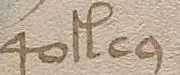
qo · k · ey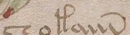
ch · o · k · aiin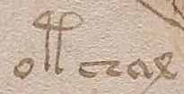
o · t · ch · al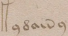
k · y · d · ain · y
qo or o, a core, often with one of the tall gallows letters, and an ending such as -ey, -aiin or -al. The split illustrates the idea, not an agreed analysis. All from folio 2r. Beinecke Rare Book & Manuscript Library, Yale University.M5. Words built from parts in fixed slots
What it is. Voynich words are not free strings of glyphs. Most can be
described as a short sequence of slots, each of which can hold only a few
glyphs, always in the same order: q only at the start, iin and y almost
only at the end, the gallows, four tall looped glyphs, in the middle.
The manuscript. John Tiltman noticed it in the 1950s and described it in 1967. Jorge Stolfi wrote it as a grammar in 2000, and Massimiliano Zattera’s slot alphabet of 2022 fits 86.6% of the running words, about half of the distinct words, to a single template of twelve slots.
What it tells apart. Natural languages constrain where letters stand too, through syllable structure, spelling and morphology, but the European languages compared with the manuscript are far less rigid; agglutinative and templatic languages have not been measured on it. A word grammar this tight is what a system of word parts or a code built from a table would produce, or a cipher that writes each letter as a group of glyphs, if those groups are chosen to fit the slots. The Naibbe cipher’s groups were chosen that way.
Caution. It is the best-established property of the text, and for exactly that reason any serious model now builds it in. Meeting it is necessary but no longer tells models apart.
M6. Word lengths
What it is. How many glyphs words have, and how the lengths are spread.
The manuscript. Narrow and symmetric, close to a binomial distribution, with very few long or very short words (Stolfi 2000). The third post shows the shape. In Ou’s test, on Takahashi’s transcription with one-letter words removed, the mean is 5.43 EVA characters (his table; his text elsewhere gives 5.25). Seven of his 18 models pass, among them the samplers that draw their words from the manuscript’s own vocabulary and so inherit its lengths.18
This figure is drawn in the browser and needs JavaScript.
Ctrl/⌘ + scroll to zoom · drag to pan · double-click to reset
What it tells apart. Natural languages usually have a long tail of long words, especially languages that build long words by inflection, agglutination or compounding. A narrow, symmetric distribution is what a word grammar with a fixed number of slots produces.
Caution. It held only conditionally in Lux’s audit, failing mainly when
uncertain spaces were closed. It also depends on how ch and iin are counted.
M7. Size of the vocabulary
What it is. How many different words appear, and how much of the text the commonest words cover.
The manuscript. 7,022 word types in 32,747 words. The 50 commonest cover 33.2% of the text. Both values are inside the range of Rozanova and Temerev’s eight prose controls: 3,454–11,041 types, and 24.0–50.3% coverage.19
This figure is drawn in the browser and needs JavaScript.
Ctrl/⌘ + scroll to zoom · drag to pan · double-click to reset
What it tells apart. At this length the vocabulary looks like a language’s: it is not unusually poor or repetitive. That troubles explanations that build the text from a small fixed stock of words. The Naibbe cipher’s vocabulary is more closed, 5.2–5.5 thousand types.
Caution. Both values depend on the length of the sample and on the space policy. Rozanova and Temerev calibrated the self-citation generator to the manuscript’s word length and type–token ratio, so for it this metric is an input (rule 7), and on its own the metric separates little.
M8. Share of word types used only once
What it is. Of all the different words in the text, how many appear just once:
The manuscript. 69.7%, or 73.0% if the uncertain spaces are closed (R&T). The eight prose controls give 46.8–67.7%, so the manuscript is just above the highest, by two points, with no published interval. If the manuscript were simply one more text like them, it would come out above all eight one time in nine by chance alone. The Naibbe cipher gives 41–42%, and the self-citation generator 59–60% on three seeds; Rozanova and Temerev found it at 57–60% whatever its settings.20
This figure is drawn in the browser and needs JavaScript.
Ctrl/⌘ + scroll to zoom · drag to pan · double-click to reset
What it tells apart. This is the sharpest single number against the two leading generators: both make the vocabulary too repetitive. It is not, on its own, an argument against language.
Caution. It moves with sample length, so it is compared only at equal length and under one recipe. The controls are eight European prose texts, with no language that builds words from many parts, which is where a high share of single-use words is expected; Rozanova and Temerev say their result should be read “not as a universal language test”. Only two generators have been measured on it under one recipe; generators that make up new words glyph by glyph have not.
M9. The slope of Zipf’s law
What it is. Rank the words from commonest to rarest and plot frequency against rank on logarithmic axes. In almost all texts the points fall close to a straight line, Zipf’s law. The slope of the line says how quickly frequency falls off.
The manuscript. Zipf’s law holds, as Gabriel Landini showed in 2001. Ou fits the slope (over the 500 commonest words in his paper; his released code fits all ranks) and finds −0.867, against −0.954 for Moby Dick and −1.124 for Cicero and Caesar, with a tolerance of ±0.10. English is inside the slope tolerance and Latin is not, but his criterion also requires the quality of the fit to be within 0.05 of the manuscript’s 0.902, and English (0.960) and Latin (0.976) both miss it, so both fail. Models that sample words by their frequency come out steeper (about −0.99); models with little structure, such as Ou’s ‘grille’ of random fragments and GPT-2, come out far shallower (about −0.3 to −0.4). Six models have a slope inside the tolerance, but only four also meet the fit criterion and pass: character-level Markov chains of orders 2 to 4 and a word-level chain of order 3. The order-5 character chain and the order-2 word chain, like English, miss on the fit.21
This figure is drawn in the browser and needs JavaScript.
Ctrl/⌘ + scroll to zoom · drag to pan · double-click to reset
What it tells apart. That Zipf’s law holds says little, because even random strings of letters and spaces come close to it, though not exactly.22 The slope is different: Ou suggests the manuscript has some mechanism, such as fixed positions for frequent words or a rule against repetition, that keeps the commonest words from dominating.
Caution. Ou found the slope stable across three transcriptions (−0.867, −0.853 and −0.852). Lux’s audit, which fits only the 100 commonest words, also found the slope stable, and flagged the property as sensitive to a quality-of-fit threshold that one file missed by 0.001.
M10, M11. Type–token ratio and word predictability
What they are. Two more of Ou’s eight measures. The standardised type–token ratio is the share of different words in fixed-length windows of text, a measure of lexical variety that does not depend on the sample length. The word-level conditional entropy is M1 for words: how uncertain the next word is given the one before.
The manuscript. On Takahashi’s transcription, a type–token ratio of 0.550 in windows of 1,000 words, against 0.475 for Moby Dick and 0.407 for Cicero and Caesar; and a word-level conditional entropy of 4.226 bits, against 4.427 and 4.433. Of Ou’s 18 models, only the best one, which is given the book’s sections, passes both.23
This figure is drawn in the browser and needs JavaScript.
Ctrl/⌘ + scroll to zoom · drag to pan · double-click to reset
What they tell apart. Together with M7 and M8, they describe the vocabulary from four sides; a model can fit one and miss another. Character-level Markov chains, which come closest overall, fail both at every order.
Caution. Ou’s preprint has not yet been peer-reviewed, and his language controls are two single works. His word entropy is a plug-in estimate on about 36,000 words and 8,500 different ones, so most word pairs occur once and the estimate falls as the vocabulary grows: uniform random text, with no link between words at all, scores 2.3 bits against the manuscript’s 4.2, and across his models the measure follows the type–token ratio. It says more about the vocabulary than about how predictable the next word is; M15 and M16 measure that directly. A wider comparison of the type–token ratio in moving windows of 2,000 words, across 101 languages in seven families, puts the manuscript in the middle of the natural range, closest to Iranian, Germanic and Romance (Bowern and Lindemann 2021, following Koen Gheuens 2019).13
M12. How few endings the words share
What it is. Count the three-glyph endings of words, and ask how many of them are needed to cover most of the text.
The manuscript. 50 endings cover 80% of the words, against 172 in Latin and 109 in German, and Currier’s A and B share a core of the same seven dominant endings (da Silva 2026).24
What it tells apart. A small set of endings is what a suffix system, a code built from a table, or a shorthand that replaces endings with a few marks would produce.
Caution. That the words share few endings is old knowledge, from Tiltman’s
beginnings and endings to Stolfi’s grammar; da Silva supplies the count. It
comes from a self-published study that has not yet been checked
independently, and no generator has been measured on it. Like M1, it depends
on whether ch and iin are counted as one glyph or several: in the author’s
own revision, merging ch and sh alone moved it from 37 endings to 50. That
is also why rule 2 requires the controls to be counted the matching way.
M13. Vocabulary that differs between parts of the book
What it is. Cut the text into five equal parts, in the order of the book, and measure how different their vocabularies are (the mean Jensen–Shannon distance, the square root of the divergence, between the parts’ word frequencies).
The manuscript. 0.535 on Takahashi’s transcription, against 0.464 for Moby Dick and 0.423 for Cicero and Caesar.25
This figure is drawn in the browser and needs JavaScript.
Ctrl/⌘ + scroll to zoom · drag to pan · double-click to reset
What it tells apart. Less than it seems. Uniformly random text, which does not change through the book at all, scores 0.568 on it in Ou’s released results, above the manuscript, and passes his test. On this post’s reading, part of any text’s value is a sampling floor: with chunks of about 7,300 words and a vocabulary of about 8,500 words, most words are rare, and rare words make any two chunks look different even if nothing changes through the book. The more single-use words a text has (M8), the higher that floor, so the manuscript’s higher value may partly be M8 again. In his released results the models that pass are uniform random text, the first-order character chain, and three of the four models given the book’s sections, each with its own vocabulary, which pass by construction.11 The opposite reading is published too: Amancio and colleagues found the manuscript’s topic words more clustered than in their languages, and took it for a compendium of different subjects, as the drawings suggest (M23).
Caution. The controls are two single works, a novel and two Latin authors; a compendium of herbal, astronomical and recipe sections in a real language is the fair control, and has not been measured. It overlaps with M23 and M24, which look at the same change of vocabulary through the book in other ways, and it assumes the present order of the leaves.
Between words
The next seven metrics ask how a word relates to its neighbours: what crosses the space between them, how much one word predicts the next, and what the spaces themselves are.
M14. Coupling across the space between words
What it is. How much the last glyph of a word tells you about the first glyph of the next. It is the mutual information
where fachys ykal ar ataiin shol, the pairs are
s–y, l–a, r–a and iin–sh.
The manuscript. 0.197 bits after correction (R&T): 0.137 in Currier’s
language A and 0.248 in B. Nearly half of it comes from a single pair, a word
ending in y followed by one beginning with q; most of the rest from r or
s followed by a, and from y avoiding a following ch or sh. Parisel,
on another transcription and glyph inventory and without the shuffle
correction, finds 0.230 bits, against 0.054–0.173 in English, French, Hebrew
and Arabic. Prescott Currier noticed the effect in 1976; Sravana Reddy and
Kevin Knight measured it in 2011, on a predictability measure that did not
separate it clearly from English;26 Emma Smith and Marco Ponzi studied it
systematically in 2019.27
What it tells apart. Prose controls are lower (0.018–0.120 bits); a catalogue of Linnaean plant records is higher (0.322). Both leading generators give almost nothing (0.006–0.009). One self-published cipher, Vitaly Averyanov’s, claims it, on his own measure rather than this one. It is a Naibbe-type cipher worked with three scribal habits: reusing recent units within the line, occasional misspelling, and, at each word boundary, drawing candidate spellings and keeping the one whose first glyph best follows the previous word’s last glyph, by a table of glyph-pair preferences; Averyanov argues the table can be estimated from inside words alone. It has not been checked independently.6 In the European prose tested, the space is where one word ends and another begins; here something carries across it. Some writing systems do record changes across the space: Sanskrit spelling writes sandhi, where a word’s last sound changes with the next word’s first, and Welsh and Irish write the mutation of a word’s first consonant after certain words. None of these was among the published controls.
This figure is drawn in the browser and needs JavaScript.
Ctrl/⌘ + scroll to zoom · drag to pan · double-click to reset
Caution. The value depends on which spaces are counted: closing the uncertain spaces lowers it to 0.162. Which of Currier’s languages carries more depends on the measure: Rozanova and Temerev find B well above A, and Currier reported the effect “almost exclusively” in B, while Parisel’s reference values put A above B (0.586 against 0.498 bits). The languages it has been compared with in print are European, Hebrew and Arabic.
This figure is drawn in the browser and needs JavaScript.
Ctrl/⌘ + scroll to zoom · drag to pan · double-click to reset
M15. How much one word predicts the next
What it is. The share of a word’s uncertainty that is removed by knowing the word before it, again after subtracting the same quantity for shuffled text. Sravana Reddy and Kevin Knight pointed out in 2011 how weak this is in the manuscript.26
The manuscript. 0.79% (R&T), between 0.48% and 0.83% when one quire at a time is left out, against 2.02–9.72% for the prose controls and 15.81% for the catalogue.28
This figure is drawn in the browser and needs JavaScript.
Ctrl/⌘ + scroll to zoom · drag to pan · double-click to reset
What it tells apart. In a natural language, grammar makes the next word much more predictable than chance. Here it hardly is, at the level of whole words. Both generators match the manuscript; the languages are well above it. Put together with M14, the dependence between adjacent words is weak but the join between them is strong: in Rozanova and Temerev’s reading, what follows depends on the glyphs at the edge, not on the word.
Caution. Most of the raw value is the bias that the shuffle removes, so the corrected estimate is small and noisy; within language A or B alone it is about zero. At this sample size it also depends on how many word types are kept: Rozanova and Temerev report it with the 2,000 commonest. With the 250 commonest the manuscript sits at 0.8 of the lowest control’s value, with 2,000 at 0.4, and with 4,000 the estimate is down at the noise floor. What they call robust is the contrast with M14, a strong edge against a weak word.
M16. Association of adjacent words
What it is. Whether particular pairs of words occur together more often than their frequencies predict (normalised pointwise mutual information). It is one of Ou’s eight.
The manuscript. 0.152, against 0.256 for Moby Dick and 0.295 for Cicero and Caesar: adjacent words are less bound to each other than in either language, which agrees with M15.29
This figure is drawn in the browser and needs JavaScript.
Ctrl/⌘ + scroll to zoom · drag to pan · double-click to reset
What it tells apart. Together with M15, it separates a text where words choose their neighbours from one where they do not. A model that copies the manuscript’s own word pairs binds words too tightly (0.306); mixing in the frequencies of single words loosens it into tolerance.
Caution. Like M10 and M11, it is one of Ou’s measures, with two single works as language controls and no interval for the manuscript. For texts in which no word pair occurs five times, Ou’s code returns 0, so the zeros of uniform random text and the grille are a default, not a measurement.
M17. Neighbours that differ by one glyph
What it is. How often two neighbouring words differ by a single glyph, as
qokedy and qokeedy do, compared with how often that happens when the words
are shuffled within the line.
The manuscript. 1.12 times the shuffled rate (R&T): such pairs are more common next to each other than by chance. The prose controls give 0.28–0.56, less than chance: all eight avoid putting near-identical words side by side. Languages that write reduplication, the repetition of a word or part of it, were not among them. The catalogue gives 2.6.30
What it tells apart. Sravana Reddy and Kevin Knight noted runs of repeated and very similar words in 2011.26 This is the effect on which Torsten Timm built his self-citation hypothesis in 2014, later developed with Andreas Schinner: a scribe who writes each new word by copying a nearby word and changing it slightly. Their generator matches it; the Naibbe cipher gives 0.82.
Caution. It rests on one study’s eight prose controls, all of which avoid near-repeats; languages that write reduplication, and record-like texts beyond the one catalogue (which exceeds the manuscript), have not been measured. Exact repeats, the same word twice running, are a related property: Gaskell and Bowern found them more frequent in the manuscript and in gibberish than in meaningful text, while Bowern and Lindemann found doubled words no more frequent than in some natural texts.
This figure is drawn in the browser and needs JavaScript.
Ctrl/⌘ + scroll to zoom · drag to pan · double-click to reset
M18. Neighbouring words alike in length
What it is. Whether a long word tends to be followed by a long word and a short one by a short one, measured as an autocorrelation (Moran’s I).
The manuscript. Positive, 0.106 to 0.172 on three versions of the transcription in Gaskell and Bowern’s released measurements, and 0.093 and 0.128 for Currier’s A and B parts; their meaningful texts run from −0.280 to +0.084, their handwritten gibberish from −0.240 to +0.226. Matlach and colleagues first reported the tendency in January 2022, as an autocorrelation of word lengths reaching up to 40 words apart; Gaskell and Bowern measured it as Moran’s I against gibberish and languages.31
This figure is drawn in the browser and needs JavaScript.
Ctrl/⌘ + scroll to zoom · drag to pan · double-click to reset
What it tells apart. Meaningful texts in Gaskell and Bowern’s study mostly give negative values; their handwritten gibberish often gives positive ones. On their measure, it is the metric that most directly favours meaningless text.
Caution. Their gibberish samples were short, one to three pages. Whether a writer keeps the habit over the whole book is not known. And Moran’s I over a whole text also counts pairs of words across line breaks, so any difference between whole lines would enter it alongside the order of words within a line. The published measurements do not try to separate the two.
M19. Parisel’s four boundary signatures
What it is. Four properties of how words begin and end, which a model must meet together, separately for Currier’s languages A and B:
- End to start. Glyphs fall into classes that prefer the ends of words and classes that prefer the starts, and in Parisel’s pooled analysis 80.6% of all junctions between words join an end-class glyph to a start-class glyph, against 19.8–35.5% in his four comparison languages. The test itself uses 71% for A and 64% for B, with ranges.
- Extremity at both ends. Some glyphs are almost never anywhere but at one
edge.
qappears 5,285 times at the start of a word and twice at the end;iin3,958 times at the end and never at the start. In his four comparison languages such extremes are rarer and have known orthographic causes, such as the final letter forms of Hebrew. - Coupling across the boundary, as in M14.
- The shape of the boundary distributions: whether the frequencies of word-initial and word-final glyphs fall off like Zipf’s law, as they do in the manuscript, rather than levelling out, as in his comparison languages.
The manuscript. As calibrated in Parisel’s paper, for A and B separately: an end-to-start rate of 71.0% for A and 64.3% for B (passing ranges 56–86% and 50–79%), glyphs at both edges, an information across the boundary of at least 0.29 and 0.25 bits, and boundary distributions that do not level out.32
This figure is drawn in the browser and needs JavaScript.
Ctrl/⌘ + scroll to zoom · drag to pan · double-click to reset
What it tells apart. A slot-based generator could not reach the coupling and the end-to-start rate together; a Cardan grille could not reach the end-to-start rate and the shape together. These are different failures from different mechanisms. Averyanov’s self-published cipher claims all four at once, with the boundary step described under M14.6 Earlier, in June 2026, a template generator posted on the voynich.ninja forum by the author of a forum thread on the four signatures was also claimed to pass them; it is unpublished.
Caution. Parisel’s comparison set is four languages, two Western European and two Semitic. Whether bilateral extremity is absent in all natural languages “cannot be determined from the present data”, as he says himself, and of the end-to-start gap: “Whether this gap would narrow for languages with richer prefix-suffix morphology (e.g., Turkish, Finnish, Swahili) or templatic structure is unknown.” He also notes that the end-to-start rate, being nearly constant, “carries almost no predictive power”. The rate depends on how the glyph classes and the glyph inventory are drawn.
This figure is drawn in the browser and needs JavaScript.
Ctrl/⌘ + scroll to zoom · drag to pan · double-click to reset
iin never occurs at the start, so its ratio is unbounded; it is drawn at its count, 3,958, as an open circle. The manuscript is the only text in which such glyphs hold both edges.M20. Two kinds of space
What it is. Transcribers mark some spaces as certain and others as uncertain. The question is whether these are really two different things on the page.
The manuscript. In boxes drawn over the page images by other researchers, uncertain spaces are narrower than certain ones (R&T). The separation is measured as an AUC of 0.905, between 0.897 and 0.913 when folios are resampled: pick an uncertain and a certain space at random, and the uncertain one is the narrower about nine times in ten. Recurring glyph groups learned from the text without any spaces also cross uncertain spaces more often. A small check on the ink itself showed the same direction, much more weakly.33
What it tells apart. If the scribe wrote two kinds of gap, any model of the text has to produce two kinds of gap. No generator has been tested on it.
Caution. The drawn boxes are themselves a human reading of the page, as Rozanova and Temerev point out.
Lines, pages and the book
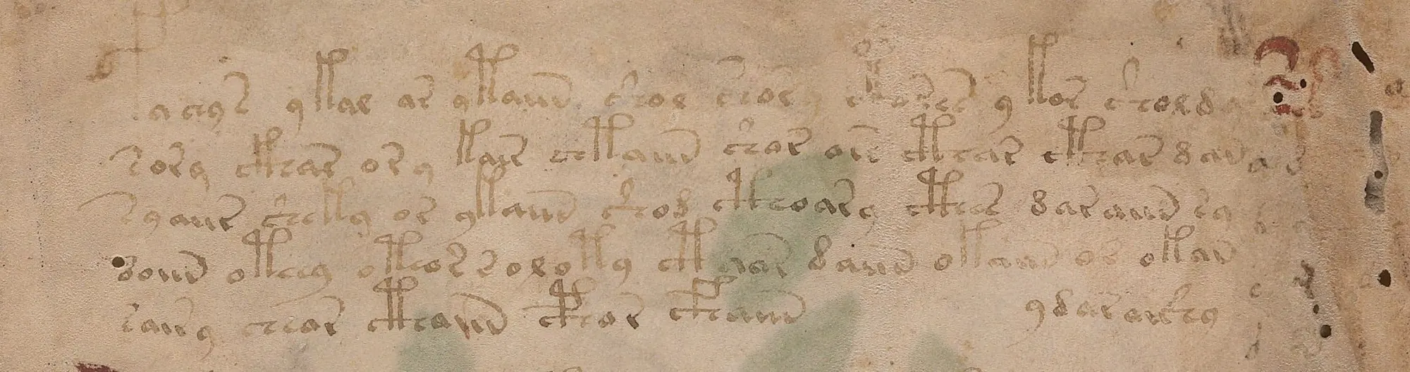 (opens the full-size image)
fachys, begins with the gallows letter f, one of the two glyphs that prefer the first line of a paragraph (M21). This page is in Currier's language A; language B (M22) differs most clearly in the glyph that follows ch and sh. Beinecke Rare Book & Manuscript Library, Yale University.M21. The line and the paragraph as units
What it is. Whether the line and the paragraph change what is written, and not only where the writing stops.
The manuscript. Strongly. Most paragraphs begin with one of the tall
gallows letters: the first lines of paragraphs open with p 24 times and with
t 12 times as often as words in the middle of lines begin with them (R&T). Two of the
gallows, p and f, are found mostly in the first lines of paragraphs, and
m and g mostly at the ends of lines. Words at the start and end of lines
differ from those in the middle. Currier wrote that in almost 25,000 words
“there is not one single case of a repeat going over the end of a line”: Three such findings convinced him, he said, “that the line is a functional entity,
(what its function is, I don’t know)”. Elmar Vogt and Patrick Feaster have
measured the effects further.34
This figure is drawn in the browser and needs JavaScript.
Ctrl/⌘ + scroll to zoom · drag to pan · double-click to reset
What it tells apart. In ordinary writing the line is where the space runs
out, and it changes words only by dividing or abbreviating one at the margin.
An explanation of the Voynich text has to know about lines. The Naibbe cipher,
by its author’s own account, does not produce this structure; Timm proposed
rules for it in 2014, which have not been measured against the list. On Gaskell
and Bowern’s measure of how letters keep to positions in the line, the
manuscript was plausibly similar both to handwritten gibberish and to
meaningful text, a weaker test than the effects above. Bowern and Lindemann
weigh two readings, a line as roughly a sentence and spelling variants that
depend on the position in the line, and treat paragraph-initial gallows and
line-final m and g as variants of ordinary words.
Caution. Some line effects are mechanical. Lines grow shorter towards the foot of a page, and Rozanova and Temerev found that this alone produces gradients in word length and glyph entropy that vanish when line length is controlled: “This is a caution for the wider line-effects literature.” A line effect counts only if it survives controlling for line length; theirs, which compare positions within the same line, do. Lux’s audit found the line-initial effect in every combination, so only its exact size depends on the recipe.
M22. Currier’s two languages
What it is. Whether the text falls into two statistically different varieties, Currier’s A and B, without being told which page is which.
The manuscript. It does. Parisel shows that the main difference is a
switch set once per page (he calls the pages folios), which governs whether
ch and sh are followed by o or by e (in his word, “the vowel”); a
two-state model assigns 195 of 197 pages with a probability above 0.8.
In Fagin Davis’s attribution the switch follows the scribe, and her scribes
work by bifolium. It was the only
claim that held in every combination of Lux’s audit. One study argues that the
whole text is a single natural language, and that A and B are not different
languages at all.3536
What it tells apart. An explanation has to produce two regimes, switched by page, inside one script and one word grammar.
Caution. The test has to be strict to mean anything. Ou’s version asks whether a classifier trained to tell A from B folios reaches about the same accuracy on synthetic text (62.1% on the manuscript, ±5 points). With 91 A and 133 B folios, always guessing B already scores 59.4%, so the manuscript’s classifier is only 2.7 points better than guessing, and any text without A/B structure passes. It is passed in his code by every model except a two-state hidden Markov model, and so separates nothing. The code also counts only a drop in accuracy as a failure: a synthetic text that is far easier to classify than the manuscript passes. The four models given the book’s sections are 32 to 37 points easier, and under the two-sided wording of his paper they would fail. Parisel’s per-page switch is the stricter target, though he finds the binary A/B label explains under a third of the variation between pages (R² = 0.293), and his switch does not match Currier’s labels on every page. A and B also overlap with sections and with hands, so a model that is told the sections has part of the answer built in.
This figure is drawn in the browser and needs JavaScript.
Ctrl/⌘ + scroll to zoom · drag to pan · double-click to reset
M23. Vocabulary that follows the subject
What it is. Whether some words cluster in particular sections or stretches of text, as topic words do in a book about several subjects.
The manuscript. They do. Marcelo Montemurro and Damián Zanette found keywords that cluster by section in 2013, and measured how much information the placement of words carries and at what scale it peaks. On that measure the manuscript is “slightly above that of English, and significantly below that of Chinese”, and peaks at a scale “very similar to that of the human language examples”, around 600 to 800 words, while their non-language controls, yeast DNA and a computer program, behave differently.37 Later work with networks of words, topic models and semantic analysis found the same clustering (Amancio and colleagues, Sterneck and colleagues, Layfield and Fagin Davis).
What it tells apart. It is usually read as a sign of meaning. Timm reads it the other way: a scribe copying nearby words produces clusters of related words without any subject.38 Gaskell and Bowern found biases in “word placement within sections” in short gibberish too, and suggest that a scribe’s gibberish “might drift considerably” over the months of writing, while granting that topic words “pose a serious challenge to proponents of the hoax hypothesis”.
Caution. The metric is solid; what it shows is disputed.
M24. Gradual drift through the book
What it is. Whether the vocabulary and the use of glyphs change gradually through the book, beyond the switch between A and B.
The manuscript. Timm has argued since 2014, most fully in 2026, that the text is “dynamic”, changing continuously as it was written, so that statistics averaged over the whole book describe no real stage of it.
What it tells apart. A static system, such as a fixed cipher table, does not drift on its own; a copying process does. A language does too, but over generations, not over the pages of one book.
Caution. Any measure of drift assumes the present order of the leaves.
One number for all metrics?
A grid of ticks and crosses is hard to rank. It is natural to ask whether the literature has a single normalised score, something like a mean squared error over all the metrics, that says how close a model comes overall. There is no agreed one. Two studies define their own, for their own sets of metrics, and two others deliberately do without.
Ou’s profile distance. Ou reports, beside the pass count, a profile distance
the mean of each metric’s deviation from the manuscript divided by that
metric’s tolerance
This figure is drawn in the browser and needs JavaScript.
Ctrl/⌘ + scroll to zoom · drag to pan · double-click to reset
The chart shows why the distance cannot replace the joint test. The two
rankings disagree: a character-level Markov chain comes closest on average,
with
Bowern and Gaskell’s Euclidean distance. In their study of ciphers and text manipulations, Claire Bowern and Daniel Gaskell put each of their 42 metrics on a common scale (z-scores) and ranked 893 comparisons by the Euclidean distance from the manuscript,
the closest thing in this literature to a root-mean-square score. They call it “a rough metric of similarity at this stage”, since the common scale makes every statistic count about equally although some are correlated. No manipulated text came as close to the manuscript as other samples of the manuscript itself.
No single number elsewhere. Gaskell and Bowern’s gibberish study judged each metric separately, by whether the distributions overlap by at least 5%, and used a classifier, not a distance, to ask which group the manuscript resembles; it came out closer to gibberish, with low confidence. Parisel, and Rozanova and Temerev, use joint pass and fail on their own profiles and no aggregate score.
Set side by side, the four ways of turning many metrics into a verdict trade different things.
| Approach | Strengths | Limits |
|---|---|---|
| Profile distance (Ou) | One number per model, so models can be ranked; scaled to the tolerances, so |
An average, so success on one metric pays for failure on another; weights are the author’s tolerances, and correlated terms (Zipf slope and fit move almost together) count more than once; mixes deviations with a test statistic on a scale about five times looser than the test, and counts the Currier gap both ways; defined only for Ou’s eight metrics |
| Euclidean distance on a common scale (Bowern and Gaskell) | Uses all 42 metrics at once; every metric weighs the same; shows at a glance which manipulations come closest | Correlated metrics count more than once, as the authors note; computed on random 200-word excerpts, so properties of long samples are measured only at that length |
| Overlap per metric, and a classifier (Gaskell and Bowern) | Each metric judged on its own, with explicit thresholds (5% overlap “plausible”, 50% “probable”); the classifier copes with correlated metrics and ranks which ones matter most | The classifier only says which of two groups the manuscript is nearer, and did so with low confidence; the gibberish samples were one to three pages long |
| Joint pass and fail (Parisel, Ou, Rozanova and Temerev) | No trade-offs: a model must meet every metric; failures point to a specific property | Binary, so it cannot tell a near miss from a wide one; the verdict depends on the tolerance chosen in advance, which in two cases of Lux’s audit decided the result |
So the answer is no: there is no standard normalised score that compares all
models across the literature. Each aggregate is defined over its own metrics,
transcription and tolerances, so a
A map of the models
A score ranks models; it does not show how they differ. Two models with the same distance from the manuscript can miss it in opposite ways. A map can show both at once: how far each model is from the manuscript, and in which direction it misses.
The two studies with full published numbers for many candidates allow one map each. They cannot share a map, because they measured different metrics on different transcriptions. Both maps are drawn the same way:
- Deviations on a common scale. For every text, each metric’s difference from the manuscript is divided by a scale. On Ou’s map the scale is his own acceptance tolerance; on Rozanova and Temerev’s, who give no tolerances, it is the spread (standard deviation) of their eight prose texts on that metric. That second choice is this post’s, not theirs.
- Distance. A text’s distance from the manuscript is its mean scaled
deviation,
- Direction. The pattern of deviations, which metrics a text misses and
in which direction, is reduced to three dimensions by principal component
analysis, which finds the few directions along which the texts’ patterns
differ most. Texts that miss the manuscript in the same way point the same
way; each text is then placed at its distance
What the maps keep and what they do not. Each text’s distance from the manuscript is exact in the three-dimensional scene, on a logarithmic scale; on a flat screen a spoke pointing towards you looks shorter, and the rings are drawn in one plane, so read distances from the tables. Directions are approximate: the tables give, for each text, how many degrees its drawn direction is from its true one. Distances between two texts on the map have no exact meaning, and the logarithmic scale shrinks those between distant texts.
Both are computed from the published numbers alone: Ou’s released results and the tables of Rozanova and Temerev.39
This figure is drawn in the browser and needs JavaScript.
Drag to rotate · Ctrl/⌘ + scroll to zoom
Texts are listed by distance from the manuscript. “Ou’s own
| # | Text | Kind | Ou’s own |
Criteria passed (of 8) | Off by | |
|---|---|---|---|---|---|---|
| 1 | Section bigram, interpolated | given the sections | 0.62 | 1.25 | 7 | 29° |
| 2 | Interpolated, smoothed | given the sections | 1.00 | 1.61 | 3 | 16° |
| 3 | Char Markov 4 | Markov chain | 1.14 | 1.07 | 3 | 10° |
| 4 | Char Markov 5 | Markov chain | 1.17 | 1.10 | 3 | 14° |
| 5 | Char Markov 3 | Markov chain | 1.22 | 1.15 | 3 | 8° |
| 6 | Char Markov 2 | Markov chain | 1.51 | 1.40 | 3 | 16° |
| 7 | Equal-split, interpolated | given the sections | 1.55 | 2.20 | 2 | 7° |
| 8 | Unigram | baseline | 1.93 | 1.78 | 3 | 6° |
| 9 | Section bigram | given the sections | 2.16 | 2.65 | 5 | 10° |
| 10 | Word Markov 1 | Markov chain | 2.43 | 2.23 | 3 | 15° |
| 11 | Word Markov 2 | Markov chain | 2.62 | 2.41 | 3 | 13° |
| 12 | LSTM | neural | 2.81 | 2.56 | 1 | 29° |
| 13 | Char Markov 1 | Markov chain | 3.07 | 2.79 | 3 | 16° |
| 14 | Word Markov 3 | Markov chain | 3.84 | 3.59 | 3 | 9° |
| 15 | English (Moby Dick) | language control | 3.92 | – | – | 61° |
| 16 | Latin (Cicero, Caesar) | language control | 4.83 | – | – | 51° |
| 17 | GPT-2 | neural | 6.37 | 5.73 | 1 | 17° |
| 18 | Uniform random | baseline | 8.47 | 7.58 | 2 | 6° |
| 19 | ‘Cardan grille’ | random fragments | 8.97 | 8.03 | 1 | 13° |
| 20 | HMM | neural | 9.79 | 8.84 | 0 | 15° |
What the first map shows:
- Nothing reaches the centre, and the closest models are those that copy
most from the manuscript. The nearest are the sampler that redraws its word
pairs within each section (
- The two languages are far away, at 3.9 for English and 4.8 for Latin, further than most of the models. The largest single part of their distance is letter entropy, more than eleven tolerances above the manuscript’s, about a third of the total. Most of Ou’s models are trained on the manuscript itself, so it is no surprise that they resemble it more closely than European prose does. The three axes are chosen by the eighteen models, which all match letter entropy, so they contain almost none of it: the languages are drawn 61° and 51° away from their true directions, and on the map they look closer to the word-level models than they are. Their distances, from the table, are exact; their positions are not.
- On two metrics the models miss in opposite directions. The word-level Markov chains and the smoothed section samplers bind adjacent words too tightly (word association too high, and plug-in word entropy too low); the character chains of orders 2 to 5 and the sampler of single words bind them too loosely. The manuscript lies between the two families on that pair. On the type–token ratio, though, both families are too varied, so neither family, nor any blend of the two, reaches it.
- The random baselines, the ‘grille’, GPT-2 and the hidden Markov model are far out, missing nearly every metric by many tolerances. Ou’s ‘grille’ joins random strings of the manuscript’s commonest fragments; it is not Rugg’s table and grille, which has not been run through the list.
This figure is drawn in the browser and needs JavaScript.
Drag to rotate · Ctrl/⌘ + scroll to zoom
Texts are listed by distance from the manuscript.
| # | Text | Kind | Off by | |
|---|---|---|---|---|
| 1 | Self-citation, seed 1 | generator | 1.52 | 3° |
| 2 | Self-citation, seed 3 | generator | 1.60 | 3° |
| 3 | Self-citation, seed 2 | generator | 1.71 | 7° |
| 4 | Italian narrative | prose | 2.30 | 9° |
| 5 | German narrative | prose | 2.41 | 5° |
| 6 | French narrative | prose | 2.51 | 5° |
| 7 | Latin botanical (Pliny) | prose | 2.52 | 11° |
| 8 | Naibbe cipher | cipher | 2.67 | 16° |
| 9 | Latin narrative | prose | 2.79 | 3° |
| 10 | Latin medical (Celsus) | prose | 2.93 | 2° |
| 11 | English herbal (Culpeper) | prose | 3.33 | 5° |
| 12 | English narrative | prose | 3.50 | 3° |
| 13 | Linnaean catalogue | catalogue | 4.91 | 11° |
What the second map shows:
- On this post’s scaling, the self-citation generator comes closest, at
- The first axis is the join between words. Coupling across the space and near-repeats together make up most of it. Prose and both generators fall short of the manuscript on this axis; the catalogue overshoots it.
- The second axis separates the generators from the languages. All of them fall short on coupling across the space, but the self-citation generator reproduces the near-repeats and the prose texts have far fewer than chance. The Naibbe cipher sits between them, pulled away also by its too few single-use words.
Both maps inherit the limits of the scores they are built on. They average, so a text that fails one metric badly can sit as close as one that fails several a little. Their scales are a choice: Ou’s tolerances on the first map, the spread of prose on the second. And a map of one study’s candidates says nothing about the candidates that study did not run.
The open targets
Some metrics on the list are not just unmet: nobody has a convincing account of why the manuscript has them at all. These are the questions the list hands to anyone with a new explanation.
- What is the line for? (M21) Currier’s question of 1976 is still unanswered. A scribe’s habit, filler at line ends, a cipher keyed to the layout, or a procedure that works line by line would each produce some line effects; none has been shown to produce these.
- What crosses the space? (M14, M20) Glyph-level coupling across word boundaries is stronger than in the prose tested, while whole words barely predict each other. A model has to make the edges of words depend on each other without making the words do so. Spelling that records sound changes across word boundaries is one candidate not yet tested in print.
- Why is the vocabulary so open? (M8) With a rigid word grammar and few endings, the text still has more single-use words than any of the eight European prose controls, and more than either generator tested.
- How does A become B? (M22) Parisel’s per-page switch describes the biggest difference, but no one has shown a transformation that carries one language into the other.
- What are the units? (M4) Rozanova and Temerev leave open whether the recurring groups are linguistic, cryptographic, palaeographic or motor: the shapes a hand falls into when writing fast.
What the harness cannot do
A harness is a filter, not an oracle. It is worth being plain about its limits.
Passing is not proof. A model that passes every metric has shown that a process of its kind could have produced the text. It has not shown that one did. A meaningless procedure and a cipher might both pass, and then the harness alone could not choose between them.
A failure rules out what was tested, not its family. A metric no generator reaches rules out those generators as built and tuned, not every generator, and not language. A metric no tested language reaches rules out a plain reading in those languages under that recipe, not a cipher or a procedure.
The metrics are not independent, and some were chosen against today’s models. Many measure overlapping things: M14 is one of Parisel’s four, and M13, M23 and M24 all measure how the vocabulary changes through the book. So “seven of eight” or “41 of 42” are not independent votes. And the metrics singled out as the sharpest are the ones current models fail; a new model designed to hit them has used them as inputs.
The values themselves can move. A benchmark value is a measurement, tied to its recipe. Three of the metrics above were rated not robust in Lux’s audit, mostly because of the tolerances chosen in advance rather than because the effects went away. A harness has to be maintained, with each value checked again when the recipe changes.
The text is not the whole object. The drawings, the layout and the order of the leaves carry information the list does not use. An explanation of the text that ignores the book it is written in is an explanation of part of the evidence. Nor does the harness ask whether a procedure was available to a scribe working on parchment of 1404–1438: a sixteenth-century grille and a cipher worked with cards are scored alike. That test lies outside the text.
What comes next
This has been a long and demanding post, but an important one. It turns fifty years of observations into quantifiable, mathematical tools: a fixed list of measurements, rules for taking them, and ways of scoring how close an explanation comes. With them in hand, different methods can now be put to work on the manuscript, to see how deep into the space of possible explanations they can reach. That is what the next posts do, with this blog’s own measurements, which have not been peer reviewed.
Footnotes
-
D. Gaskell and C. Bowern, “Gibberish after All? Voynichese Is Statistically Similar to Human-Produced Samples of Meaningless Text”, and C. Bowern and D. Gaskell, “Enciphered after All?”, both in Proceedings of the International Conference on the Voynich Manuscript 2022, CEUR-WS 3313. The companion paper finds the word-level statistics compatible with some kinds of cipher too. Their word-length measure (M18) is Moran’s I; its values here are from their released metrics (see the note to M18). Some of the volunteers, a 2019 class and the authors, knew the manuscript’s statistical properties before writing, and all wrote in the Latin alphabet; the authors report that leaving out the authors’ own samples did not change their results. ↩
-
C. Parisel, “Evidence of Layered Positional and Directional Constraints in the Voynich Manuscript: Implications for Cipher-Like Structure”, arXiv:2604.19762, and “A Quantitative Confirmation of the Currier Language Distinction”, arXiv:2604.25979 (2026), preprints. The positional counts in M19 and the page switch in M22 are from these. ↩
-
Y. Ou, “A Statistical Turing Test for the Voynich Manuscript: Evaluating Eight Quantitative Linguistic Properties Across Nine Generative Model Families”, preprint (Research Square, May 2026), doi:10.21203/rs.3.rs-9755825/v1. Its eight measures are M1, M6, M9, M10, M11, M13, M16 and M22 of the list. ↩
-
L. Rozanova and A. Temerev, “A Glyph Is Not a Letter, a Token Is Not a Word, a Space Is Not a Space: What the Units of Voynichese Are Not”, arXiv:2608.17096 (2026), preprint. The values marked R&T, and those for the two generators and their controls in the scorecard, are from their Tables 3, 4, 6, 7 and 11 and §3.3 and §3.8. ↩
-
D. R. Amancio, E. G. Altmann, D. Rybski, O. N. Oliveira Jr. and L. da F. Costa, “Probing the Statistical Properties of Unknown Texts: Application to the Voynich Manuscript”, PLOS ONE 8/7 (2013), e67310, doi:10.1371/journal.pone.0067310. The two exceptions are in their Table 4: the number of repeated word pairs, and the intermittency of the commonest words. ↩
-
The models: M. A. Greshko, “The Naibbe Cipher: A Substitution Cipher That Encrypts Latin and Italian as Voynich Manuscript-Like Ciphertext”, Cryptologia (online 26 November 2025), doi:10.1080/01611194.2025.2566408, whose author acknowledges that it does not produce the line and paragraph structure; T. Timm and A. Schinner, “A Possible Generating Algorithm of the Voynich Manuscript”, Cryptologia 44/1 (2020), 1–19, doi:10.1080/01611194.2019.1596999, after T. Timm, “How the Voynich Manuscript Was Created”, arXiv:1407.6639 (2014), which proposes rules for paragraph openings and line positions; G. Rugg, “An Elegant Hoax? A Possible Solution to the Voynich Manuscript”, Cryptologia 28/1 (2004), 31–46, for the grille, and G. Rugg and G. Taylor, “Hoaxing Statistical Features of the Voynich Manuscript”, Cryptologia 41/3 (2017; online 2016), 247–268, doi:10.1080/01611194.2016.1206753; V. Averyanov, “A Workshop Cipher: A Generative Model Reproducing the Statics and Dynamics of the Voynich Manuscript Text” (Zenodo, September 2026), doi:10.5281/zenodo.22874156, self-published and not independently checked in print. The sources of the list: W. R. Bennett Jr., Scientific and Engineering Problem-Solving with the Computer (1976); J. Tiltman, “The Voynich Manuscript: ‘The Most Mysterious Manuscript in the World’”, NSA Technical Journal 12/3 (1967); J. Stolfi, “A Grammar for Voynichese Words” and “On the VMS Word Length Distribution” (2000); M. Zattera, “A New Transliteration Alphabet Brings New Evidence of Word Structure and Multiple ‘Languages’ in the Voynich Manuscript”, CEUR-WS 3313 (2022); G. Landini, “Evidence of Linguistic Structure in the Voynich Manuscript Using Spectral Analysis”, Cryptologia 25/4 (2001), 275–295; F. J. F. da Silva, “Sub-lexical Regularity in the Voynich Manuscript” (Zenodo, 2026), doi:10.5281/zenodo.20546419 (version 3.0), self-published; E. M. Smith and M. Ponzi, “Glyph Combinations across Word Breaks in the Voynich Manuscript”, Cryptologia 43/6 (2019), 466–485; V. Matlach, B. A. Janečková and D. Dostál, “The Voynich Manuscript: Symbol Roles Revisited”, PLOS ONE 17/1 (2022), e0260948; E. Vogt, “The Line as a Functional Unit in the Voynich Manuscript: Some Statistical Observations” (2012, self-published); P. Feaster, “Rightward and Downward Grapheme Distributions in the Voynich Manuscript”, CEUR-WS 3313 (2022); P. Currier, papers of 1976, transcribed at voynich.nu; M. A. Montemurro and D. H. Zanette, “Keywords and Co-Occurrence Patterns in the Voynich Manuscript: An Information-Theoretic Analysis”, PLOS ONE 8/6 (2013), e66344; D. R. Amancio et al., “Probing the Statistical Properties of Unknown Texts: Application to the Voynich Manuscript”, PLOS ONE 8/7 (2013), e67310; R. Sterneck, A. Polish and C. Bowern, “Topic Modeling in the Voynich Manuscript”, arXiv:2107.02858 (2021); C. Layfield and L. Fagin Davis, “The Application of Latent Semantic Analysis to the Voynich Manuscript”, Digital Humanities Quarterly 20/1 (2026), doi:10.63744/2ezxpskcezq4. ↩ ↩2 ↩3
-
V. Lux, “How Stable Are Quantitative Claims about Voynichese? A Cross-Transliteration and Representation-Sensitivity Audit” (Zenodo, September 2026), doi:10.5281/zenodo.22850758; preregistered, self-published and not peer reviewed. ↩
-
R. Kinnison, “The Voynich Manuscript’s Positional Entropy Collapse: Comparative Evidence from Languages and Ciphers”, Cryptologia (online 7 September 2026), 1–18, doi:10.1080/01611194.2026.2697318. His cipher control is his own construction on the Naibbe pattern, applied to Latin. The values here are as in his preprint of December 2025. ↩
-
L. Fagin Davis, “How Many Glyphs and How Many Scribes? Digital Paleography and the Voynich Manuscript”, Manuscript Studies 5/1 (2020), 164–180, doi:10.1353/mns.2020.0011; T. Timm, “One Hand, Five Labels: A Critical Examination of the Five-Scribe Hypothesis for the Voynich Manuscript” (Zenodo, 2026), doi:10.5281/zenodo.19169450, self-published. ↩
-
C. Layfield and L. Fagin Davis, “Singulion Structure and the Voynich Manuscript”, Digital Medievalist 19 (2026), doi:10.4000/16k0a. What is disputed is its reconstruction of the original arrangement; that the present order is not the original is widely accepted. ↩
-
Ou’s paper, his tables and his released results (github.com/yangou2012/voynich_stt, commit 6d061eb) do not always agree; this post follows the released results, which match his pass counts. In them the Currier criterion is one-sided, an accuracy drop of less than 5 points, while the paper says the accuracy must deviate by less than 5 points; the four section models are 32 to 37 points more accurate than on the manuscript, so they pass in the code and would fail as the paper words it, leaving his best model at six of eight. On M13 the paper says that every stationary model fails, while the released results list uniformly random text and the first-order character chain as passing. His Table 4 lists the first-order character chain as failing M13, and implies that the smoothed section model passes word association; the released results say the opposite in both cases. His abstract says that every model has a steeper Zipf slope than the manuscript, which his own results contradict for eight of his 18 models: the grille, GPT-2, the hidden Markov model, random text, the character chains of orders 1 to 3 and the order-3 word chain. His paper decides each criterion on at least 15 of 30 runs; his code, followed here, decides on the mean of the 30. ↩ ↩2 ↩3
-
Ou’s paper describes letter and word entropy as judged by a Kolmogorov–Smirnov test too; his released code instead requires the mean over 30 runs to be within 0.10 bits of the manuscript’s value, and keeps the Kolmogorov–Smirnov test for the distribution of word lengths, passing a model when the mean of its 30 p-values exceeds 0.05. Averaging p-values is not a valid test, and with about 36,000 words in each sample the test’s 5% critical value is about 0.010, a fifth of the 0.05 his distance uses as its scale. A pass means only that the averaged test did not reject. ↩
-
L. Lindemann and C. Bowern, “Character Entropy in Modern and Historical Texts: Comparison Metrics for an Undeciphered Manuscript”, arXiv:2010.14697 (2020). Their 2.11 and 2.48 bits are on Takahashi’s transcription, with EVA strokes as glyphs and with common clusters merged; they note that frequent digraphs, such as Venda vh, are among the languages’ predictable letter pairs. C. Bowern and L. Lindemann, “The Linguistics of the Voynich Manuscript”, Annual Review of Linguistics 7 (2021), 285–308, give the comparison of type–token ratios across language families. ↩ ↩2
-
Rozanova and Temerev, Table 6 (2.69 bits and 6.45 effective choices for the manuscript; 3.45–3.52 bits and 10.91–11.50 choices for the four controls) and §3.7 (2.43 bits with transitions inside words only). Lindemann and Bowern, p. 27 (2.11 and 2.48 bits; 2.77–6.14 for the Wikipedia languages) and the caption of their Figure 10 (Hawaiian 2.77, Venda 2.79, Tswana 2.82); the quotation is from p. 23. ↩
-
M. D. Owens, “Voynichese Has Natural-Language-Range Character Entropy but Anomalous Order-Scaling: A Corrected Statistical Characterization”, Knowledge Commons (version 2, July 2026), doi:10.17613/asz1z-nax02, self-published. It uses held-out, smoothed models of up to three glyphs of context, not the
-
Kinnison’s preprint: medial positional entropy and ΔBPC for the whole manuscript in Takahashi’s transcription, p. 16 (2.11 bits, 0.30), and in Friedman’s, Currier’s and Stolfi’s, pp. 17–18 (2.01, 2.08 and 2.19 bits; 0.31, 0.29 and 0.25); the recipes section, p. 14 (1.95); his four language controls, pp. 19–20 (3.08–3.16 bits; ΔBPC 0.51–0.78); his Naibbe cipher of Latin, p. 21 (2.01 bits, 0.34). ↩ ↩2
-
Rozanova and Temerev, pp. 15–16 (the minimum at 64 merges, with 88 unit types of mean span 2.39 symbols; 32 when the merges are learned without the quire scored) and Table 7 (the self-citation generator’s 0.65–0.86 at 64 merges, against the manuscript’s 1.05). ↩
-
Ou, §3.2 and Table 2 (mean 5.43), printed p. 11 (mean 5.25), and Table 4 (seven of 18 models pass); his released results give the distribution plotted here and a mean of 5.25. ↩
-
Rozanova and Temerev, Table 3 and p. 9; the Naibbe cipher’s 5,234 and 5,463 types, for its Caesar and Pliny ciphertexts, from Appendix A.5. ↩
-
Rozanova and Temerev, Table 3 (69.7%, 73.0%, and 46.8–67.7% for the controls), Table 7 and Appendix A.5 (the Naibbe cipher 40.5% and 41.7%, the self-citation generator 59–60% on three seeds), and A.5 for “57–60% singletons for every setting”; the quotation is from p. 20. ↩
-
Ou, §3.2 (the fit over the 500 commonest words; R² 0.902), Table 1 (−0.867, −0.954 and −1.124), Table 2 (the tolerance) and Table 3 (−0.867, −0.853 and −0.852 on three transcriptions). The models’ slopes, and the quality of fit for English (0.960) and Latin (0.976), are from his released results. ↩
-
W. Li, “Random Texts Exhibit Zipf’s-Law-Like Word Frequency Distribution”, IEEE Transactions on Information Theory 38/6 (1992), 1842–1845, doi:10.1109/18.165464; R. Ferrer-i-Cancho and B. Elvevåg, “Random Texts Do Not Exhibit the Real Zipf’s Law-Like Rank Distribution”, PLOS ONE 5/3 (2010), e9411, doi:10.1371/journal.pone.0009411. ↩
-
Ou, Table 1 (type–token ratio 0.550, 0.475 and 0.407; word entropy 4.226, 4.427 and 4.433 bits) and Table 4 (passes). ↩
-
F. J. F. da Silva, “Sub-lexical Regularity in the Voynich Manuscript: BPE Morpheme Signature Discriminates Competing Hypotheses and Reveals a Concentrated Suffix System”, Zenodo, version 3.0 (2026), doi:10.5281/zenodo.20546419, as stated in its abstract; self-published. It is one version of a record (concept doi:10.5281/zenodo.20356422) whose version 2.0 gave 37 endings, before
chandshwere merged. ↩ -
Ou, Table 1 (0.535, 0.464 and 0.423), §3.2 (five chunks of 7,275 tokens; acceptance by the mean absolute deviation of the matrix) and Table 3 (a vocabulary of 8,474 types); passes from his released results. ↩
-
S. Reddy and K. Knight, “What We Know About the Voynich Manuscript”, Proceedings of the 5th ACL-HLT Workshop on Language Technology for Cultural Heritage, Social Sciences, and Humanities (2011), 78–86. ↩ ↩2 ↩3
-
Rozanova and Temerev, Table 4 and Table 11 (0.197 bits; A 0.137 and B 0.248; 0.162 with the uncertain spaces closed; 0.018–0.120 for the prose controls, 0.322 for the catalogue, 0.006–0.009 for the generators) and p. 10 (the share carried by
ybeforeq). Parisel, Table 3 (0.230 bits, and 0.054–0.173 for his four languages). ↩ -
Rozanova and Temerev, Table 3 (0.79%; 2.02–9.72% for the prose controls, 15.81% for the catalogue), p. 9 and Appendix A.4 (0.48–0.83% with one quire left out; about zero within A or B), pp. 10–11 (the dependence on the number of word types kept), and Table 7 (the generators). ↩
-
Ou, Table 1 (0.152, 0.256 and 0.295), printed p. 11 and Table 5 (0.306 for the section-bigram model, 0.145 with interpolation). ↩
-
Rozanova and Temerev, Table 4 and Table 11 (1.12; 0.28–0.56 for the prose controls; 2.57 for the catalogue; 0.82 for the Naibbe cipher). ↩
-
Gaskell and Bowern’s released metrics, github.com/danielgaskell/voynich (commit d076a7d,
results/metrics_paperv1.csv, checked against its SHA-256 sum), columnwordlen_autocorr, and their Figure 3. Their “Voynichese” group is three versions of the transcription (EVA Basic, EVA Full and Claston’s v101) and the Currier A and B parts of EVA Basic. ↩ -
Parisel, Table 2 (80.6%, and 19.8–35.5% for the four languages), §4.1.1 (the counts for
qandiin) and Table 1 (the reference values for A and B, 71.0% and 64.3%, and their ranges). ↩ -
Rozanova and Temerev, §3.4: the gaps, the AUC of 0.9053 with its folio-resampled interval of 0.8972 to 0.9127, and 176 of 179 folios wider at certain spaces. ↩
-
Rozanova and Temerev, §3.6 (p 24-fold and t 12-fold; f 5-fold and k 3-fold). Currier’s words are from P. H. Currier, “Some Important New Statistical Findings”, in M. E. D’Imperio (ed.), New Research on the Voynich Manuscript: Proceedings of a Seminar (1976), transcribed at voynich.nu. ↩
-
R. V. Ponnaluri, “The Voynich Manuscript Was Written in a Single, Natural Language”, Cryptologia 49/6 (2025; online 2024), 505–524, doi:10.1080/01611194.2024.2414128. ↩
-
Parisel, “A Quantitative Confirmation of the Currier Language Distinction”, §5.1 and Table 8 (195 of 197 folios above 0.8); Ou, §3.2 (62.1% and the ±5-point criterion); his released baseline gives 91 A and 133 B folios; the models’ accuracies are from his released results. Parisel’s R² of 0.293 is from his §3.6 and Table 5. ↩
-
M. A. Montemurro and D. H. Zanette, “Keywords and Co-Occurrence Patterns in the Voynich Manuscript: An Information-Theoretic Analysis”, PLOS ONE 8/6 (2013), e66344, doi:10.1371/journal.pone.0066344; the comparison is in their Figure 1B and the text beside it. ↩
-
T. Timm, “Co-Occurrence Patterns in the Voynich Manuscript”, arXiv:1601.07435 (2016), and “The Challenge of Analyzing a Dynamic Text: Why the Voynich Manuscript Resists Conventional Interpretation”, Cryptologia (online 7 September 2026), 1–18, doi:10.1080/01611194.2026.2693462. ↩
-
Ou’s values are his released results at github.com/yangou2012/voynich_stt (commit 6d061eb), checked by their SHA-256 sums; those for Rozanova and Temerev are from their Tables 3, 7 and 11 and Appendix A.5, with each self-citation seed’s coupling across the space from Table 11. The principal component analysis is run on the deviation profiles scaled to unit length, without centring, so that the manuscript stays at the origin and near and far texts weigh equally in choosing the axes; the share kept is the mean over texts of the squared cosine between each profile and its drawn direction. Three further properties: the radius is a mean of absolute deviations while the direction comes from profiles scaled to unit length, which keeps the radius exact; the word-length and parts-of-the-book terms are unsigned, so every text lies on one side of those directions; and Ou’s models are means of 30 runs, whose spread is not shown. Ou’s released value for his language controls on the parts of the book was computed against his superseded named-section matrix (mean 0.584) rather than the positional one the models are scored against (0.535); their matrices are not released, so the maps use the gap between the means, a lower bound. The construction preserves distances between texts only roughly: their rank correlation with the true distances is 0.98 on Ou’s map with a linear radius and 0.83 with the logarithmic one drawn, and 0.96 on the second map. Classical multidimensional scaling of the same distances would keep them better (Kruskal stress 0.044 against 0.099 on Ou’s map, 0.050 against 0.117 on the second), at the cost of the manuscript’s place at the origin and of exact distances from it. ↩